Tetanus sero data

Concentration

library(tidyverse)
library(gt)
library(mgcv)

all_tetanus <- readRDS("data/preprocessed/all_samples.rds")

There is currently no specific threshold to classify tetanus serostatus, for this analysis, a conservative threshold of 0.1IU/ml is used.

# threshold to be considered positive
positive_threshold <- 0.1

Preprocess data

Label whether it is oucru or hcdc sample
Label the collection period for samples from each source
Compute rounded age
Compute concentration
- Use median value to compute where available, use lower or upper otherwise
- Concentration is computed by titer*dilution_fct where titer is the predicted “concentration” from the standard curve.
Label whether the sample is considered positive using 0.1IU/ml threshold
- If concentration is not available –> the OD is either too high or too low, in which case seropositivity is determined by which extreme it is closer to (i.e., if OD closer to 0, label as negative and label as positive when OD is closer to 4)

Also filter samples from HCMC only

Code for preprocessing data

preprocessed_data <- all_tetanus %>% 
  mutate(
    log_concentration = case_when(
      !is.na(median) ~ median,
      !is.na(upper) ~ upper,
      !is.na(lower) ~ lower,
      .default = NA
    ),
    concentration = (10^log_concentration)*dilution_factors,
    serostatus = if_else(
      !is.na(concentration),
      # if concentration available, determine positivity using threshold
      if_else(concentration >= 0.1, "positive", "negative"),
      # if concentration not available, determine positivity using OD
      # if result closer to OD upper bound, it is positive
      if_else((4 - result) < (result - 0), "positive", "negative")
    ),
    source = if_else(str_detect(sample_id, "^U"), "hcdc", "oucru"),
    age = case_when(
      !is.na(dob) ~ as.double(difftime(date_collection, dob, unit = "days"))/365.25,
      !is.na(exact_age) ~ exact_age, 
      !is.na(age_min) ~ age_min,
      !is.na(age_max) ~ age_max,
      .default = NA
    ),
    rounded_age = round(age)
  ) %>% 
  filter(
    province %in% c("HCMC", "Hồ Chí Minh", "HỒ CHÍ MINH")
  ) %>% group_by(source) %>% 
  mutate(
    time_durr = paste0(
      format(min(date_collection), "%Y/%m"), 
      " - ", 
      format(max(date_collection), "%Y/%m"))
  ) %>% 
  ungroup()

Different dilutions

Visualize distribution of concentration at different dilution levels and the positive threshold

Plot distribution of log concentration at different dilutions

preprocessed_data %>% 
  ggplot() +
    geom_density(
      aes(
        x = concentration,
        color = time_durr
      )
    ) +
    geom_vline(
      aes(
        xintercept = positive_threshold
      ),
      color = "green",
      linetype = "dashed"
    ) +
    scale_x_log10() +
    facet_wrap(~ dilution_factors) +
    labs(
      color = "Collection period"
    )

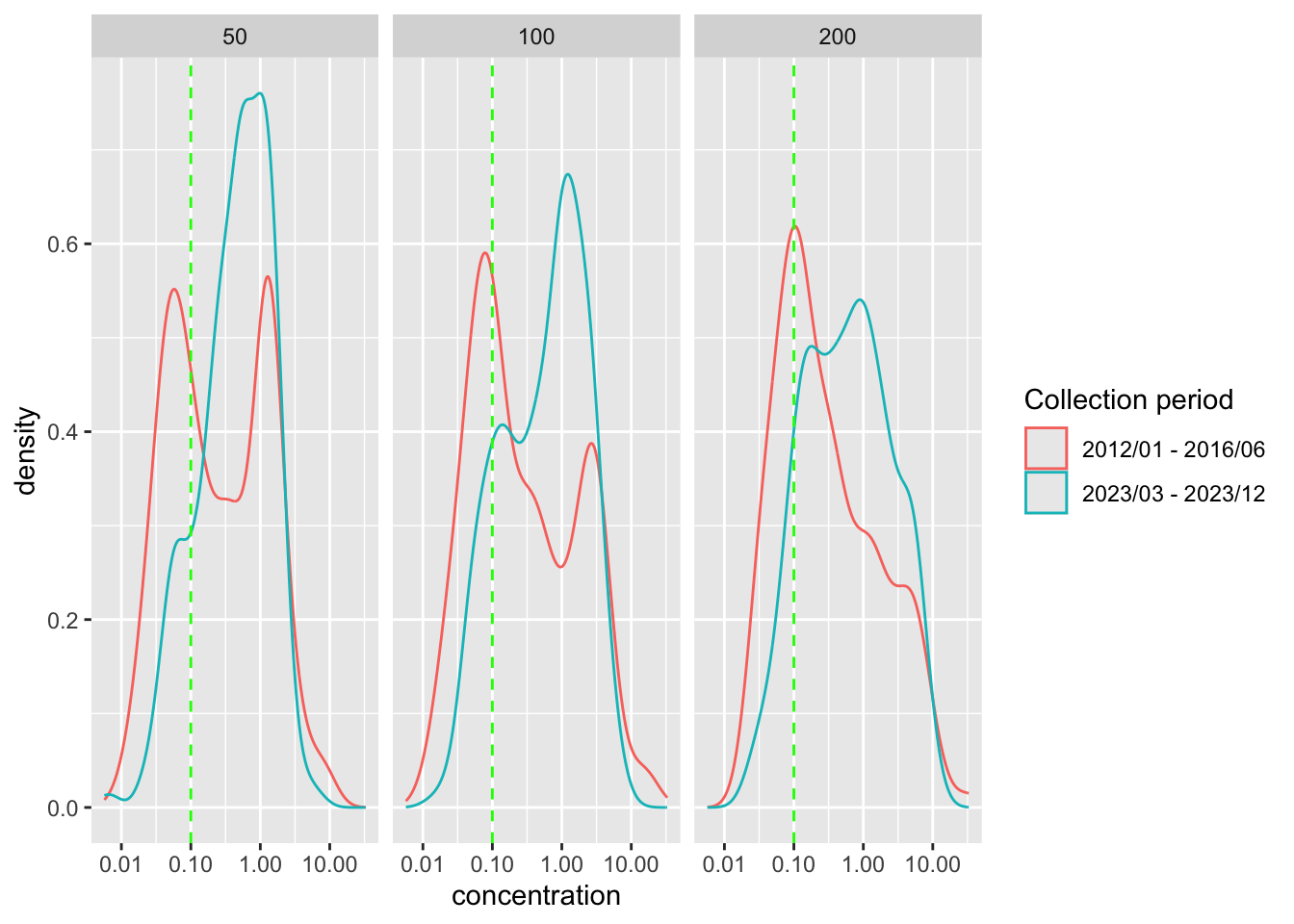
# which dilution factor for the following analyses
dilution_fct <- 200

Concentration by collection period

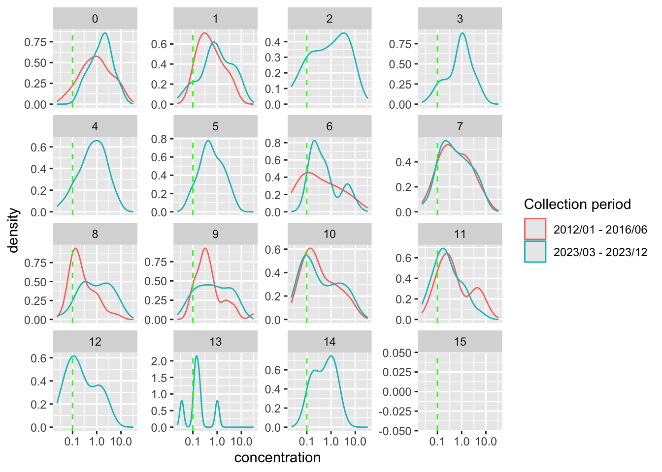
Distribution of concentration for each age group

Plot distribution of concentration stratified by age

preprocessed_data %>% 
  filter(
    rounded_age <= 15,
    dilution_factors == dilution_fct
    ) %>% 
  ggplot() +
    geom_density(
      aes(
        x = concentration,
        color = time_durr
      )
    ) +
    geom_vline(
      aes(xintercept = positive_threshold),
      color = "green",
      linetype = "dashed"
    ) +
    scale_x_log10()+
    facet_wrap(~ rounded_age, scales = "free_y") + 
    labs(
      color = "Collection period"
    )

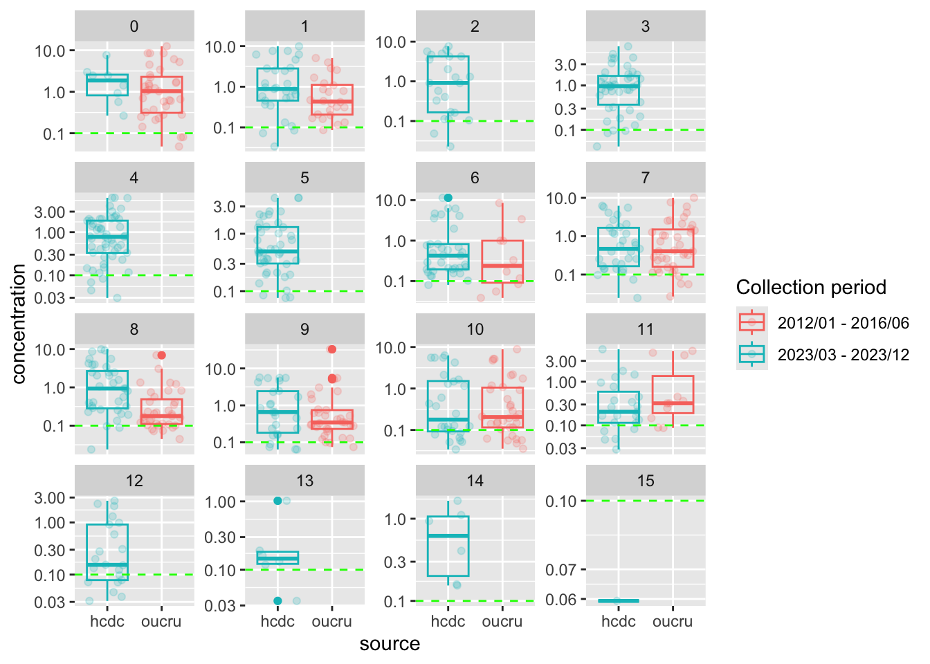
Box plot of concentration per age group

Code for box plot of concentration

preprocessed_data %>% 
  filter(
    rounded_age <= 15,
    dilution_factors == dilution_fct
    ) %>% 
  ggplot() +
    geom_jitter(
        aes(
          x = source,
          y = concentration,
          color = time_durr
        ),
        alpha = 0.2
      ) +
    geom_boxplot(
      aes(
        x = source,
        y = concentration,
        color = time_durr
      ),
      fill = NA
    ) +
    geom_hline(
      aes(yintercept = positive_threshold),
      color = "green",
      linetype = "dashed"
    ) +
    scale_y_log10()+
    facet_wrap(~ rounded_age, scales = "free_y")+
    labs(
        color = "Collection period"
      )

Code for plotting concentration over age

preprocessed_data %>% 
  filter(
    rounded_age <= 15,
    dilution_factors == dilution_fct
    ) %>% 
  ggplot() +
    geom_point(
          aes(
            x = age,
            y = concentration,
            color = time_durr
          ),
          alpha = 0.2
        ) +
    geom_smooth(
        aes(
          x = age,
          y = concentration,
          color = time_durr,
          fill = time_durr
        ),
        method = "loess"
      ) +
    geom_hline(
      aes(yintercept = positive_threshold),
      color = "green",
      linetype = "dashed"
    ) +
    scale_y_log10() +
    labs(
        color = "Collection period"
      ) + 
    guides(fill = "none")

`geom_smooth()` using formula = 'y ~ x'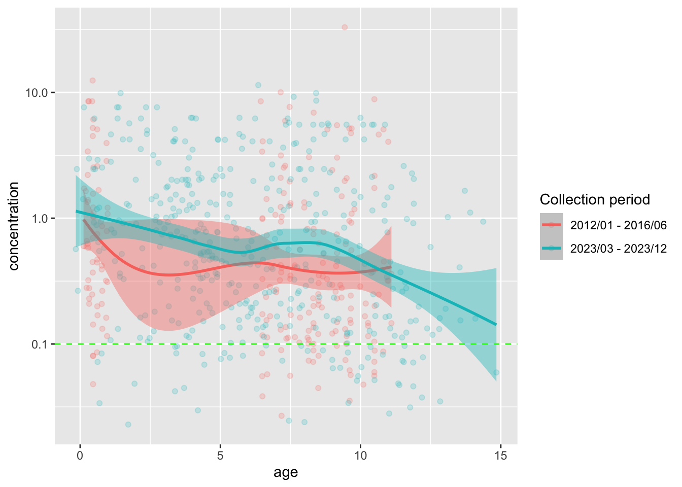

Note:

There are no samples for age groups 3 - 5 and 12 - 15 during the 2012-2016 collection period

The following table summarizes number of samples for each rounded age from each collection period

Check sample size for each age-group

preprocessed_data %>% 
  filter(
    rounded_age <= 15,
    dilution_factors == dilution_fct
    ) %>% 
  group_by(time_durr, rounded_age) %>% 
  count() %>% 
  pivot_wider(
    names_from = time_durr,
    values_from = n
  ) %>% 
  arrange(rounded_age)

# A tibble: 16 × 3
# Groups:   rounded_age [16]
   rounded_age `2012/01 - 2016/06` `2023/03 - 2023/12`
         <dbl>               <int>               <int>
 1           0                  36                  10
 2           1                  25                  39
 3           2                  NA                  28
 4           3                  NA                  54
 5           4                  NA                  63
 6           5                  NA                  46
 7           6                  11                  41
 8           7                  39                  37
 9           8                  35                  42
10           9                  34                  30
11          10                  35                  31
12          11                  11                  25
13          12                  NA                  22
14          13                  NA                   6
15          14                  NA                   6
16          15                  NA                   1

Stratified by age group

Separate the data into 2 age groups: <3 and 7-12 for comparison

Compute age group for stratification

data_by_agegrp <- preprocessed_data %>%
  mutate(
    age_group = case_when(
      age < 3 ~ "< 3",
      age >= 7 & age <= 12 ~ "7-12",
      .default = NA
    )
  ) %>% 
  filter(
    !is.na(age_group),
    dilution_factors == dilution_fct
  )

Perform two samples Wilcoxon test to compare distribution of concentration (on log scale) of 2 age groups (<3, 7-12) between samples from 2 collection periods

Perform wilcoxon test to compare log concentration for 2 age groups

concentration_by_agegrp <- data_by_agegrp %>% 
  filter(!is.na(concentration)) %>% 
  group_by(
    age_group
  ) %>% 
  nest() %>% # divide the data.frame by each age group
  mutate(
    # perform t.test to compare samples from each source
    # t_test = map(data, 
    #   ~ t.test(
    #     log_concentration ~ source, data = .x
    #   )
    # ),
    # p_value = map_dbl(t_test, ~.x$p.value),
    # perform two-sample wilcoxon test instead to compare samples from each source
    wilcox = map(data, 
      ~ t.test(
        log_concentration ~ time_durr, data = .x
      )
    ),
    p_value = map_dbl(wilcox, ~.x$p.value),
    # compute summary for samples from each source (HCDC and OUCRU)
    dat_summary = map(data, \(dat){
      dat %>% 
        group_by(time_durr) %>% 
        summarize(
          median_concentration = median(concentration),
          lwr = quantile(concentration, probs = 0.25),
          upper = quantile(concentration, probs = 0.75)
        ) %>% 
        mutate(
          label = sprintf("%.4f (%.4f–%.4f)",
          median_concentration,
          lwr,
          upper),
          .keep = "unused"
        )
    }
    )
  ) %>% 
  unnest(
    dat_summary
  ) %>% 
  pivot_wider(
    names_from = time_durr,
    values_from = label
  )

Generate the comparison table

concentration_by_agegrp %>%
  select(-wilcox, -data) %>% 
  relocate(p_value, .after = last_col()) %>% 
  ungroup() %>% 
  gt(rowname_col = "age_group") %>%
  tab_header(title = "Log(concentration) by collection period and age group") %>% 
  tab_style(
    style = list(cell_text(weight = "bold")),
    locations = list(
      cells_column_labels(everything()), 
      cells_stub()
    )
  )

	2012/01 - 2016/06	2023/03 - 2023/12	p_value
Log(concentration) by collection period and age group
< 3	0.6785 (0.2746–1.6855)	0.9333 (0.3935–2.8357)	0.3767952
7-12	0.3187 (0.1287–1.0571)	0.4078 (0.1331–1.7665)	0.2340958

Note:

The result suggests that for both age groups, there is no statistically significant difference in the log(concentration) of samples between the 2 collection periods.

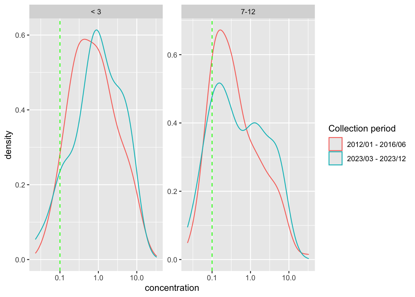
The following plots demonstrate the distribution of log(concentration)

Density plot
Box plot

Generate the density plot

concentration_by_agegrp %>%
  unnest(data) %>% 
  ggplot() +
    geom_density(
      aes(
        x = concentration,
        color = time_durr
      )
    ) +
    geom_vline(
      aes(xintercept = positive_threshold),
      color = "green",
      linetype = "dashed"
    ) +
    scale_x_log10() +
    facet_wrap(~ age_group, scales = "free_y") +
    labs(
        color = "Collection period"
      )

Generate the box plot

concentration_by_agegrp %>%
  unnest(data) %>% 
  ggplot() +
    geom_jitter(
        aes(
          x = time_durr,
          y = concentration,
          color = time_durr
        ),
        alpha = 0.2
      ) +
    geom_boxplot(
      aes(
        x = time_durr,
        y = concentration,
        color = time_durr
      ),
      fill = NA
    ) +
    geom_hline(
      aes(yintercept = positive_threshold),
      color = "green",
      linetype = "dashed"
    ) +
    scale_y_log10() +
    labs(
        color = "Collection period"
      ) +
    facet_wrap(~ age_group, scales = "free_y")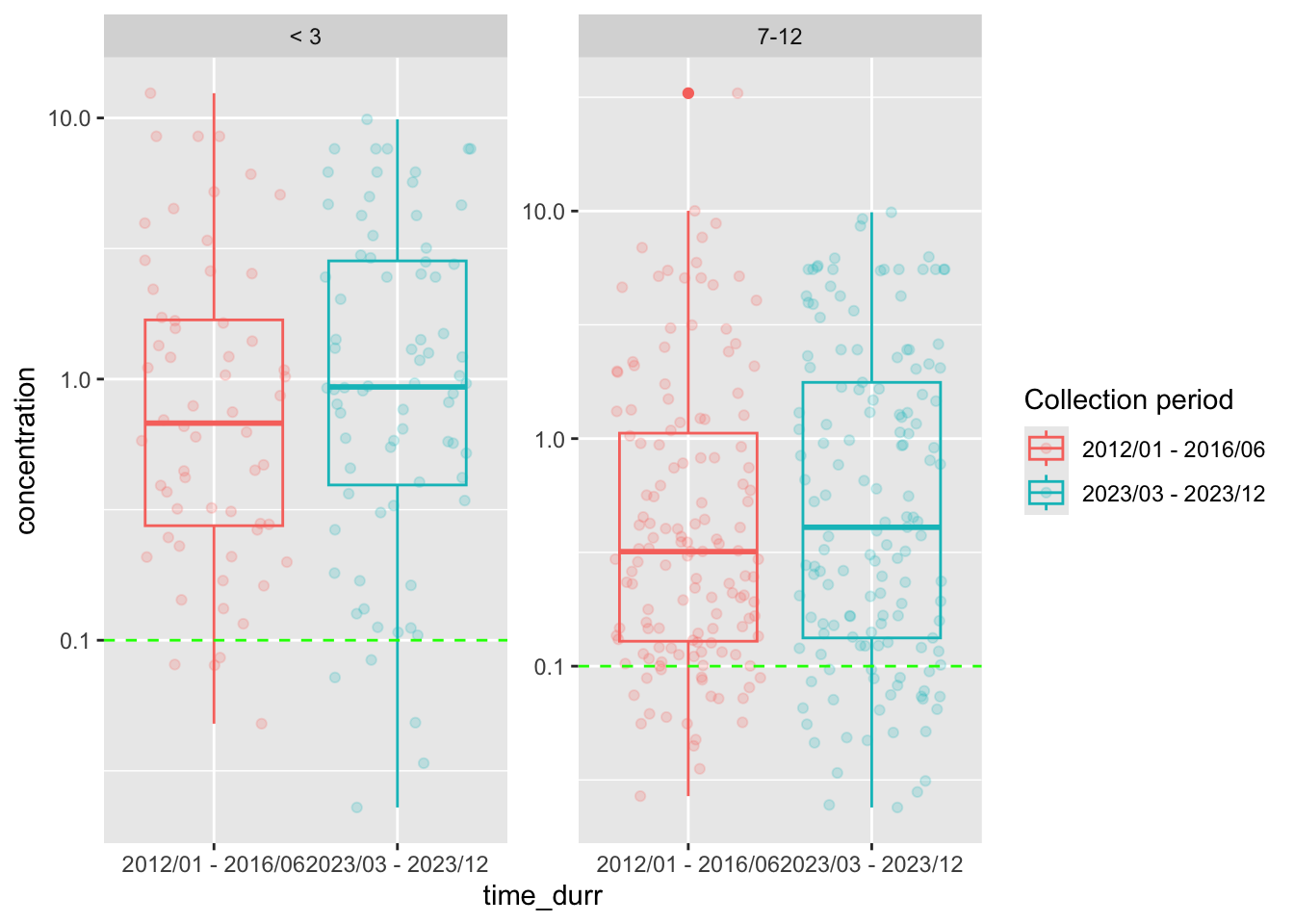

Seroprevalence

Comparison table

Compute prevalence and confidence interval

prevalence_by_agegrp <- data_by_agegrp %>% 
  group_by(
    time_durr, age_group
  ) %>% 
  summarize(
    seropositive = sum(serostatus == "positive"),
    sample_size = sum(!is.na(serostatus))
  ) %>% 
  rowwise() %>% 
  mutate(
    seroprevalence = seropositive/sample_size,
    seroprevalence_ci = list(
      prop.test(
      x = seropositive, n = sample_size,
      conf.level = 0.95)$conf.int
    ),
    seroprevalence_lwr = seroprevalence_ci[[1]],
    seroprevalence_upper = seroprevalence_ci[[2]]
  ) %>% 
  ungroup()

Seroprevalence with confidence intervals

generate the table

prevalence_by_agegrp %>%
  mutate(
    label = sprintf("%.1f%% (%.1f–%.1f%%)",
        100 * seroprevalence,
        100 * seroprevalence_lwr,
        100 * seroprevalence_upper)
  ) %>% 
  select(time_durr, age_group, label) %>%
  pivot_wider(names_from = time_durr,
              values_from = label) %>%
  gt(rowname_col = "age_group") %>%
  tab_header(title = "Seroprevalence by collection period and age group") %>% 
  tab_style(
    style = list(cell_text(weight = "bold")),
    locations = list(
      cells_column_labels(everything()), 
      cells_stub()
    )
  )

	2012/01 - 2016/06	2023/03 - 2023/12
Seroprevalence by collection period and age group
7-12	85.8% (78.7–90.9%)	83.4% (76.6–88.6%)
< 3	93.4% (83.3–97.9%)	94.0% (86.9–97.5%)

Comparison tables with p-value. Only samples from the 2 age groups <3 and 7-12 are included.

Overall
By age group

Chi-squared test

generate the summary table

library(gtsummary)

data_by_agegrp %>% 
  select(serostatus, time_durr) %>% 
  tbl_summary(
    by = time_durr,          
    type = all_categorical() ~ "categorical",
    missing = "no"
  ) %>%
  add_p(test = everything() ~ "chisq.test") %>%  
  add_n() %>%                                    
  bold_labels()

Characteristic	N	2012/01 - 2016/06 N = 202¹	2023/03 - 2023/12 N = 263¹	p-value²
serostatus	465			>0.9
negative		24 (12%)	33 (13%)
positive		178 (88%)	230 (87%)
¹ n (%)
² Pearson’s Chi-squared test

perform Fisher exact test

prevalence_compare <- data_by_agegrp %>% 
  group_by(
    age_group
  ) %>% 
  nest() %>% # divide the data.frame by each age group
  mutate(
    # perform fisher.test to compare samples from each source
    fisher_test = map(data, 
      \(df){
        tab <- table(df$serostatus, df$time_durr)
        fisher.test(tab)
      }
    ),
    fisher_test_p = map_dbl(fisher_test, ~.x$p.value),
    odd_ratio = map_chr(fisher_test, \(out){
      sprintf("%.3f (%.3f–%.3f)",
        out$estimate,
        out$conf.int[1],
        out$conf.int[2])
    }),
    # compute summary for samples from each source (HCDC and OUCRU)
    dat_summary = map(data, \(dat){
      dat %>% 
        group_by(time_durr) %>% 
        summarize(
          label = paste0(sum(serostatus == "positive"), "/", n())
        )
    }
    )
  ) %>% 
  unnest(
    dat_summary
  ) %>% 
  ungroup() %>% 
  pivot_wider(
    names_from = time_durr,
    values_from = label
  )

Check the negative-positive counts for each age group

map(prevalence_compare$data, 
  \(df){
    table(df$serostatus, df$time_durr)
})

[[1]]
          
           2012/01 - 2016/06 2023/03 - 2023/12
  negative                 4                 6
  positive                57                94

[[2]]
          
           2012/01 - 2016/06 2023/03 - 2023/12
  negative                20                27
  positive               121               136

Comparison table with p-value from the Fisher exact test

generate the table

prevalence_compare %>%
  select(-data, -fisher_test) %>%
  relocate(odd_ratio, fisher_test_p, .after = last_col()) %>% 
  rename(
    p_val = fisher_test_p,
    `2023/03 - 2023/12 (pos/tot)` = `2023/03 - 2023/12`,
    `2012/01 - 2016/06 (pos/tot)` = `2012/01 - 2016/06`,
    `Odd ratio (95% CI)` = odd_ratio
  ) %>% 
  gt(rowname_col = "age_group") %>%
  tab_header(title = "Compare prevalence by collection period and age group") %>% 
  tab_style(
    style = list(cell_text(weight = "bold")),
    locations = list(
      cells_column_labels(everything()),
      cells_stub()
    )
  ) %>%
  fmt_number(
    columns = where(is.numeric),
    decimals = 4
  )

	2012/01 - 2016/06 (pos/tot)	2023/03 - 2023/12 (pos/tot)	Odd ratio (95% CI)	p_val
Compare prevalence by collection period and age group
< 3	57/61	94/100	1.099 (0.218–4.862)	1.0000
7-12	121/141	136/163	0.833 (0.420–1.631)	0.6344

Age stratified seroprevalence

Helper function to compute age-stratified aggregated seroprev

compute_seroprev <- function(data, age_lim, dilution_fct, group_var){
  if(!is.null(group_var)){
    out <- data %>% 
      filter(age<=age_lim, dilution_factors == dilution_fct) %>% 
      mutate(
        serostatus = if_else(serostatus == "positive", 1, 0),
        !! group_var := factor(.data[[group_var]])
      ) %>% 
      group_by(rounded_age, .data[[group_var]]) %>% 
      summarize(
        pos = sum(serostatus, na.rm = TRUE),
        tot = n(),
        neg = tot - pos,
        seroprev = sum(serostatus, na.rm = TRUE)/n()
      ) %>% 
      ungroup()
  }else{
    out <- data %>% 
      filter(age<=age_lim, dilution_factors == dilution_fct) %>% 
      mutate(
        serostatus = if_else(serostatus == "positive", 1, 0)
      ) %>% 
      group_by(rounded_age) %>% 
      summarize(
        pos = sum(serostatus, na.rm = TRUE),
        tot = n(),
        neg = tot - pos,
        seroprev = sum(serostatus, na.rm = TRUE)/n()
      ) %>% 
      ungroup()
  }
  
  out
}

Check whether there is a difference in seroprevalence between:

samples from the 2 collection periods
female and male samples

Model stratified by collection period

# ----- Model with smoothing stratified by collection period ------
seroprev_mod_coll <- preprocessed_data %>% 
  compute_seroprev(age_lim = 15, dilution_fct = dilution_fct, group_var = "time_durr") %>% 
  gam(cbind(pos, neg) ~ s(rounded_age, bs = "bs", by = time_durr) + time_durr, data = ., family=binomial(link = "logit"))
summary(seroprev_mod_coll)


Family: binomial 
Link function: logit 

Formula:
cbind(pos, neg) ~ s(rounded_age, bs = "bs", by = time_durr) + 
    time_durr

Parametric coefficients:
                           Estimate Std. Error z value Pr(>|z|)    
(Intercept)                  1.8778     0.2000   9.389   <2e-16 ***
time_durr2023/03 - 2023/12   0.1184     0.2581   0.459    0.646    
---
Signif. codes:  0 '***' 0.001 '**' 0.01 '*' 0.05 '.' 0.1 ' ' 1

Approximate significance of smooth terms:
                                            edf Ref.df Chi.sq  p-value    
s(rounded_age):time_durr2012/01 - 2016/06 1.000  1.000  2.369 0.123779    
s(rounded_age):time_durr2023/03 - 2023/12 2.854  3.555 19.386 0.000406 ***
---
Signif. codes:  0 '***' 0.001 '**' 0.01 '*' 0.05 '.' 0.1 ' ' 1

R-sq.(adj) =  0.355   Deviance explained = 54.4%
UBRE = 0.33797  Scale est. = 1         n = 24

Model stratified by gender

# ----- Model with smoothing stratified by gender ------
seroprev_mod_gender <- preprocessed_data %>% 
  compute_seroprev(age_lim = 15, dilution_fct = dilution_fct, group_var = "gender") %>% 
  gam(cbind(pos, neg) ~ s(rounded_age, bs = "bs", by = gender) + gender, data = ., family=binomial(link = "logit"))
summary(seroprev_mod_gender)


Family: binomial 
Link function: logit 

Formula:
cbind(pos, neg) ~ s(rounded_age, bs = "bs", by = gender) + gender

Parametric coefficients:
            Estimate Std. Error z value Pr(>|z|)    
(Intercept)   2.2626     0.2973   7.611 2.73e-14 ***
gendermale   -0.3301     0.3328  -0.992    0.321    
---
Signif. codes:  0 '***' 0.001 '**' 0.01 '*' 0.05 '.' 0.1 ' ' 1

Approximate significance of smooth terms:
                              edf Ref.df Chi.sq  p-value    
s(rounded_age):genderfemale 1.000  1.000  0.044    0.835    
s(rounded_age):gendermale   2.809  3.503 24.448 4.35e-05 ***
---
Signif. codes:  0 '***' 0.001 '**' 0.01 '*' 0.05 '.' 0.1 ' ' 1

R-sq.(adj) =  0.439   Deviance explained = 54.3%
UBRE = 0.19118  Scale est. = 1         n = 29

Model without stratification for smoothing

# ----- Baseline model (no stratification) ------
seroprev_mod <- preprocessed_data %>% 
  compute_seroprev(age_lim = 15, dilution_fct = dilution_fct, group_var = NULL) %>%
  gam(cbind(pos, neg) ~ s(rounded_age, bs = "bs"), data = ., family=binomial(link = "logit"))
summary(seroprev_mod)


Family: binomial 
Link function: logit 

Formula:
cbind(pos, neg) ~ s(rounded_age, bs = "bs")

Parametric coefficients:
            Estimate Std. Error z value Pr(>|z|)    
(Intercept)   1.9015     0.1342   14.17   <2e-16 ***
---
Signif. codes:  0 '***' 0.001 '**' 0.01 '*' 0.05 '.' 0.1 ' ' 1

Approximate significance of smooth terms:
                 edf Ref.df Chi.sq  p-value    
s(rounded_age) 1.669  2.087  18.36 0.000139 ***
---
Signif. codes:  0 '***' 0.001 '**' 0.01 '*' 0.05 '.' 0.1 ' ' 1

R-sq.(adj) =  0.478   Deviance explained = 61.5%
UBRE = 0.089952  Scale est. = 1         n = 16

Note:

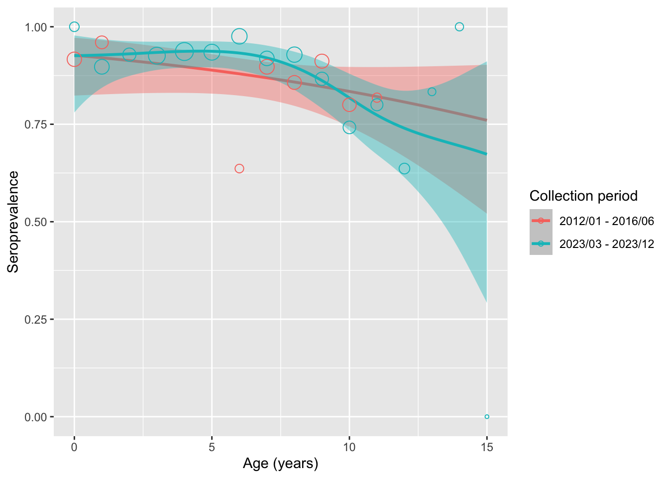
The result from model stratified by (sample) source suggests that:

There’s no statistically significant difference in seroprevalence between the samples from these 2 sampling period

The result from model stratified by gender suggests that:

There’s no statistically significant difference in seroprevalence between male and female samples

However, it may be due to the fact that the sample size for the earlier collection period (using OUCRU samples) is quite small and we don’t have any data for several age groups (3-6, 11-14)

Another issue is that there is an imbalance in the number of male vs female samples during later collection period (male:female ratio is 13.58:1)

preprocessed_data %>% 
  filter(dilution_factors == dilution_fct) %>% 
  group_by(source, time_durr, gender) %>% 
  count()

# A tibble: 4 × 4
# Groups:   source, time_durr, gender [4]
  source time_durr         gender     n
  <chr>  <chr>             <chr>  <int>
1 hcdc   2023/03 - 2023/12 female    33
2 hcdc   2023/03 - 2023/12 male     448
3 oucru  2012/01 - 2016/06 female   241
4 oucru  2012/01 - 2016/06 male     247

Quick visualization

Visualize the model for collection period/gender stratified smoothing

Helper function to visualize model with confidence interval

visualize_pred <- function(data, mod, group_var, ci = 0.95, length_out = 100, cex = 20){
  
  if(!is.null(group_var)){
    newdata <- data %>% 
      select({{group_var}}) %>% 
      distinct() %>% 
      crossing(
        rounded_age = seq(min(data$rounded_age), max(data$rounded_age), length.out = length_out)
      )
  }else{
    newdata <- data.frame(
      rounded_age = seq(min(data$rounded_age), max(data$rounded_age), length.out = length_out)
    )
  }
  
  linkinv <- mod$family$linkinv
  p <- (1 - ci) / 2
  n <- mod$df.residual
  
  out <- predict(
    mod,
    newdata = newdata, se.fit = TRUE) %>% 
  as_tibble() %>% 
  select(fit, se.fit) %>% 
  mutate(
    rounded_age = newdata$rounded_age,
    
    lower = linkinv(fit + qt(p, n) * se.fit),
    upper = linkinv(fit + qt(1 - p, n) * se.fit),
    fit = linkinv(fit)
  )
  
  if(!is.null(group_var)){
    out <- out %>% 
      mutate(
        !! group_var := newdata[[group_var]]
      )
  }
  
  ggplot() +
    geom_smooth(
      aes(
        x = rounded_age, y = fit, 
        ymin = lower, ymax = upper,
        color = if(!is.null(group_var)) factor(.data[[group_var]]) else "cornflowerblue",
        fill = if(!is.null(group_var)) factor(.data[[group_var]]) else "cornflowerblue"
      ),
      data = out,
      stat = "identity"
    ) +
    geom_point(
      aes(
        x = rounded_age, y = seroprev, 
        size = cex*pos/max(tot), 
        color = if(!is.null(group_var)) factor(.data[[group_var]]) else "black",
        fill = if(!is.null(group_var)) factor(.data[[group_var]]) else "grey"
      ),
      shape = 1,
      data = data
    ) +
    guides(size = "none", fill="none") +
    labs(x = "Age (years)",
         y = "Seroprevalence",
         color = if(!is.null(group_var)) str_to_title(group_var) else "") 
}

Collection period
Gender

preprocessed_data %>% 
  compute_seroprev(age_lim = 15, dilution_fct = dilution_fct, group_var = "time_durr") %>%
  visualize_pred(mod = seroprev_mod_coll, group_var = "time_durr") +
  labs(
    color = "Collection period"
  )

Imbalance in sample size causes larger CI interval for female

preprocessed_data %>% 
  compute_seroprev(age_lim = 15, dilution_fct = dilution_fct, group_var = "gender") %>% 
  visualize_pred(mod = seroprev_mod_gender, group_var = "gender")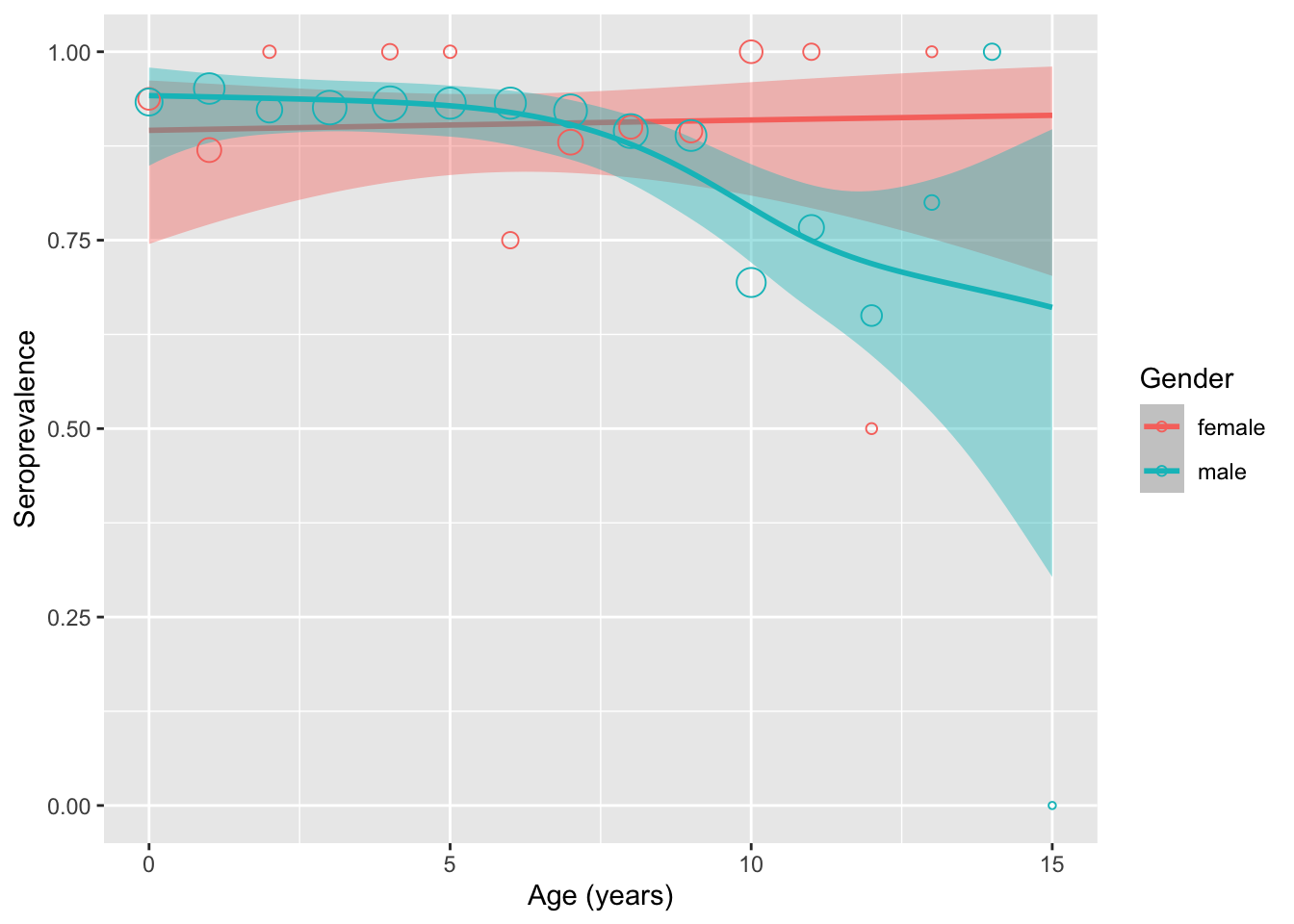

HCDC samples - a closer look

Seroprevalence - FOI by age

Age-stratified seroprevalence across HCDC samples

library(serosv)

# use rounded age
preprocessed_data %>% 
  filter(
    source == "hcdc", 
    rounded_age <= 15,
    dilution_factors == dilution_fct,
    !is.na(serostatus)
  ) %>% 
  select(rounded_age, serostatus) %>% 
  mutate(
    status = if_else(serostatus == "positive", 1, 0)
  ) %>%
  rename(
    age = rounded_age
  ) %>% 
  penalized_spline_model(s = "tp", framework = "pl") %>% 
  plot()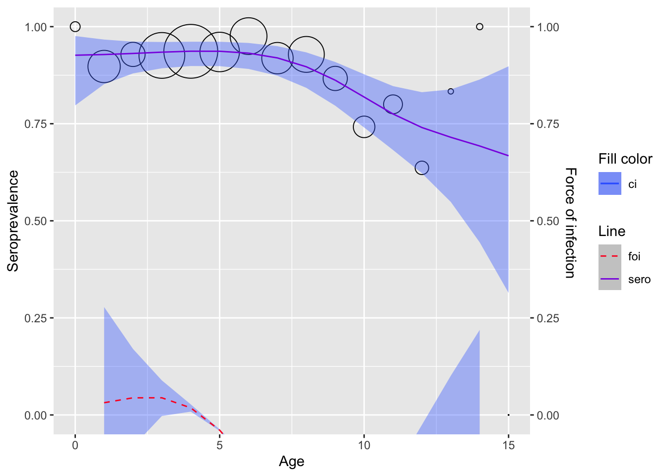

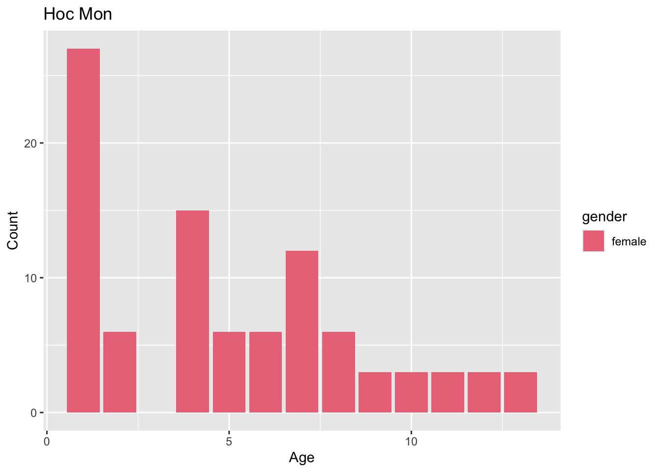
Sample distribution by district

preprocessed_data %>% 
  filter(source == "hcdc") %>% 
  generate_district_plots() %>% 
  pull(age_gender_plot)

[[1]]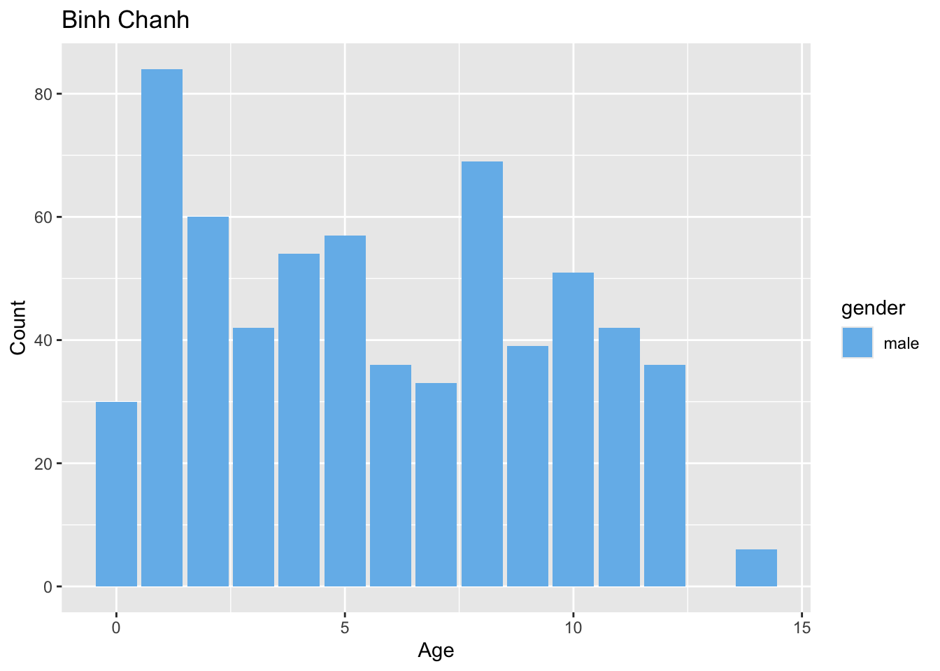


[[2]]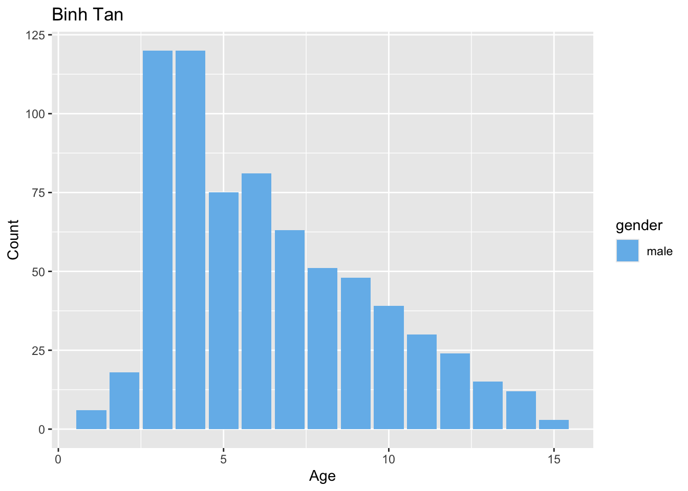


[[3]]


[[4]]